Neural Rendering Adventures #1: NeRFs

22 Sep, 2025

In my last blog post, I discussed digitally modeling humans, particularly using parametric models. If you're curious about the general approach to designing parametric models and how they work, feel free to read about it here.

One of the interesting things we can achieve with these parametric models is to optimize their parameters with respect to one or multiple images of a person to match their appearance. This handles reasonably well the geometry part of the things, but there is also a need to deal with the texture of the model, the hair and the face. Most of the time, we need neural rendering approaches to differentiably render the model. This allows us to optimize both geometry and appearance aspects like clothing and hair texture. It's only natural we cover some of the foundational work that has been published in the area of Neural Rendering to understand this kind of pipeline.

While there are many applications of Neural Rendering for digital humans, I'll focus on three key topics that have dominated recent research:

Neural Radiance Fields (NeRFs)
Gaussian Splatting
Differentiable Rendering

Neural Radiance Fields

In this section, we'll focus on the main idea of NeRFs and explore code snippets that will enable you to write a full training loop for a NeRF. The seminal NeRF paper was published in 2020, in the deep learning world, that is ancient. There have been many improvements since then, but the core concept remains valuable. NeRFs are primarily used to synthesize novel views of scenes by optimizing a neural representation of the scene as a continuous volume. NeRFs revolutionized the field by how they represent a scene by not using meshes or point clouds.They also showcased NeRF's strength in capturing view-dependent effects, which was rare at that point.

The main idea is simple: the volume is represented as an MLP. The input to this MLP is the (x,y,z) coordinate of where you are sampling the volume and the (θ, φ) viewing direction of the ray. These viewing direction parameters are what allow the NeRF to learn view-dependent appearances of the scene. The output from the MLP is 4-dimensional: (R, G, B, σ) where σ is the density (or opacity) value. 5e700a025ff238947d682a1f_pipeline_website-03

The second important part of the paper is the positional encoding they employ. MLPs are not great at representing high-frequency details, which is a prevalent problem when applying machine learning to computer graphics. So instead of directly supplying the (x,y,z, θ, φ) coordinates to the network, they apply positional encoding, borrowed from the Transformer architecture, to each component separately. Specifically, they encode the spatial coordinates x and the three components of the Cartesian viewing direction unit vector d. This encoding transforms each coordinate using sine and cosine functions at different frequencies, enabling the network to capture fine-grained spatial details.

γ (p) = (\sin (2^{0} π p), \cos (2^{0} π p), \dots, \sin (2^{L - 1} π p), \cos (2^{L - 1} π p))

Now we know what goes into the MLP and what comes out of it. You might be asking right now, "That seems simple, is that all?" And that would be a good question because there's a bit more nuance to the main idea. Just providing the viewing direction and location wouldn't be enough to train a volumetric representation of the scene. The color of a ray passing through the scene is rendered by borrowing from classical volume rendering formulation. The formula might look intimidating, but we'll break it down piece by piece.

C (𝐫) = \int_{t_{n}}^{t_{f}} T (t) σ (𝐫 (t)) 𝐜 (𝐫 (t), 𝐝) d t, where T (t) = \exp (- \int_{t_{n}}^{t} σ (𝐫 (s)) d s)

So the color of the ray is represented as $C (r)$ , which is an integral between the near and far bounds $t_{n}$ and $t_{f}$ . The ray is represented as $r (t) = o + t d$ , where o is the origin and d is the direction. This is called a parametric representation of a ray. Let's go through the terms in the integral:

T(t): The transmittance at point t along the ray. This represents how much light can pass through the volume up to that point without being absorbed or scattered. It's the probability that the ray travels from $t_{n}$ to $t$ without hitting anything.
σ(r(t)): The volume density at 3D position $r (t)$ . It can be interpreted as the differential probability of a ray terminating at an infinitesimal particle at location $r (t)$ . We want the network to learn this to represent how "opaque" or "dense" the medium is at that point. Higher density means more light absorption/scattering.
c(r(t), d): The emitted color at 3D position $r (t)$ when viewed from direction d. This is also learned by the network and captures the view-dependent appearance (like specular reflections!).

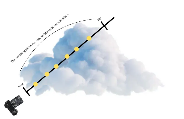
Let’s try to build a simple intuition of what this formula represents. We can think of this formulation as marching the ray through the volumetric representation and accumulating color contributions from each point, but also weighting the contributions by how much light can actually reach that point and how much light that point emits toward the camera. In which case points behind dense regions contribute less because the transmittance is lower.

Near

Since this formula involves a continuous integral over the ray, we cannot compute it exactly on a digital computer. We need to discretize it. In the paper, the authors numerically estimate this continuous integral using quadrature. To put it simply, quadrature is a technique to evaluate a continuous integral numerically. We replace the continuous integral with a weighted sum over a finite amount of samples along our range. Instead of using a deterministic quadrature and limiting the MLP’s resolution, they split the range $[t_{n}, t_{f}]$ into $N$ evenly-spaced bins and then draw one sample uniformly at random from each bin. This stratified random sampling helps prevent aliasing artifacts that could occur with regular sampling patterns:

t_{i} ~ 𝒰 [t_{n} + \frac{i - 1}{N} (t_{f} - t_{n}), t_{n} + \frac{i}{N} (t_{f} - t_{n})]

Hence the continuous integral formulation can now be written as a weighted sum of these finite amount of points:

\hat{C} (𝐫) = \sum_{i = 1}^{N} T_{i} (1 - \exp (- σ_{i} δ_{i})) 𝐜_{i}, where T_{i} = \exp (- \sum_{j = 1}^{i - 1} σ_{j} δ_{j})

Once again, let’s break down the formulation term by term to understand what exactly is going on:

$T_{i}$ : The cumulative transmittance at sample $i$ . The probability that light travels from the ray start to sample $i$ , without being absorbed or scattered along the way.
$σ_{i}$ : Volume density at sample point $i$ .
$δ_{i}$ : Distance between adjacent samples ( $δ_{i} = t_{(} i + 1) - t_{i}$ ).
$(1 - e x p (- σ_{i} δ_{i}))$ : Alpha compositing weight. The probability that the ray terminates at sample $i$ .
$c_{i}$ : Emitted color at sample point $i$ .

With these in mind: We check how much light reaches the point ( $T_{i}$ ), see how much of it gets absorbed or scattered $(1 - e x p (- σ_{i} δ_{i}))$ , and add that sample's color contribution. This is essentially alpha compositing that is used in computer graphics for blending transparent layers front-to-back.

In even simpler terms, you can think of stacking colored transparent sheets: each sheet contributes its color to the final result, and with each additional sheet, less light can pass through. The sheets closer to your eye have more influence on the final color you see.

Optimizing the NeRF

The authors use a clever technique to make sampling more efficient. Instead of using a single MLP, they use two: one for "coarse" sampling and one for "fine" sampling. This hierarchical approach is commonly used in graphics algorithms and high-performance computing. Since spending computational power on empty and occluded space is inefficient, they first sample $N_{c o a r s e}$ points and evaluate the coarse network. Then they sample $N_{f i n e}$ additional points, biased toward regions with higher density or opacity values that likely contain actual scene content.

The loss function is quite simple as well. It's simply the total squared error between the rendered and ground truth pixel colors for both the coarse and fine renderings:

ℒ = \sum_{𝐫 \in ℛ} [{‖ {\hat{C}}_{c} (𝐫) - C (𝐫) ‖}_{2}^{2} + {‖ {\hat{C}}_{f} (𝐫) - C (𝐫) ‖}_{2}^{2}]

The authors have a great visualization for the loss, that is quite intuitive:

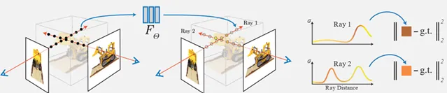
We simply shoot rays starting from a pixel of an input image, sampling the volume representation along the way and using alpha compositing to summarize and calculate the color seen from that pixel. You can think of this as looking through a very small window toward an object and reporting the color you see. Then we can compare the color we've accumulated with the actual color from the image in our dataset. I'm a big fan of approaches where the loss formulation ends up being such a simple operation in the end.

The authors reported a whopping 1-2 days of training time for this approach back in the day. Thankfully, the researchers at NVIDIA came up with an enormous improvement over this approach with their Instant-NGP paper. They sped up the optimization by several orders of magnitude, reducing training time from days to minutes. They achieved this through a novel multiresolution hash encoding that dramatically reduces the computational requirements.

Coding Parts of the Pipeline

I always understand concepts better when I can code the network and its main operations myself. So let's implement the most important parts of NeRF. Let's start by implementing the positional encoding function. This directly follows the formula we discussed in the previous sections.

def positional_encoding(x: torch.Tensor, L=10, include_original=False):
  encoding = []
  if include_original:
    encoding = [x]
  
  for i in range(L):
      freq = 2.0 ** i
      encoding.append(torch.sin(freq * math.pi * x))
      encoding.append(torch.cos(freq * math.pi * x))

  return torch.cat(encoding, dim=-1)

If we run the following code, we'll see that our 3-dimensional coordinates get encoded into a 60-dimensional vector.

X = torch.tensor([1, 2 ,3])
encoded = positional_encoding(X, L=10)
print(encoded.shape)

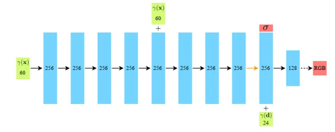
The authors use L=10 for the Cartesian coordinates and L=4 for the viewing direction, resulting in a 60-dimensional input for positions and a 24-dimensional vector for the viewing direction.

Now let's implement the MLP. The structure of the network is quite simple, it's essentially a well-designed MLP with skip connections. In the diagram below, black arrows indicate layers with ReLU activation, orange arrows represent layers with no activation, dashed arrows show sigmoid activation, and "+" indicates vector concatenation. The density value is output by one of the intermediate layers, while the RGB values are output by the final layer.

network

class NeRF(nn.Module):
    def __init__(self, pos_dim=63, dir_dim=27, hidden_dim=256):
        super().__init__()
       
        self.pos_layers = nn.ModuleList([
            nn.Linear(pos_dim, hidden_dim),
            nn.Linear(hidden_dim, hidden_dim),
            nn.Linear(hidden_dim, hidden_dim),
            nn.Linear(hidden_dim, hidden_dim),
            nn.Linear(hidden_dim + pos_dim, hidden_dim),
            nn.Linear(hidden_dim, hidden_dim),
            nn.Linear(hidden_dim, hidden_dim),
            nn.Linear(hidden_dim, hidden_dim)
        ])
       
        self.density_head = nn.Linear(hidden_dim, 1)
        self.feature_head = nn.Linear(hidden_dim, hidden_dim)
       
        self.dir_layer = nn.Linear(hidden_dim + dir_dim, hidden_dim // 2)
        self.color_head = nn.Linear(hidden_dim // 2, 3)
       
        self.relu = nn.ReLU()
        self.sigmoid = nn.Sigmoid()
   
    def forward(self, pos_enc, dir_enc):
        x = pos_enc
       
        for i, layer in enumerate(self.pos_layers):
            if i == 4:
                x = torch.cat([x, pos_enc], dim=-1)
            x = self.relu(layer(x))
       
        density = self.relu(self.density_head(x))
        features = self.feature_head(x)
       
        dir_input = torch.cat([features, dir_enc], dim=-1)
        dir_features = self.relu(self.dir_layer(dir_input))
        color = self.sigmoid(self.color_head(dir_features))
       
        return color, density

Now we need to create our inputs to the network. We require positions and viewing directions of the samples, then we can run them through our network. The complete pipeline involves several steps: generate rays from the image dataset pixels, sample points along the rays using stratified sampling, feed these points to the MLP to get per-sample (RGB, σ) results, and finally use the volume rendering function we discussed to create the final predicted pixel color. Fortunately, all these steps can be implemented using PyTorch operations, so we can leverage PyTorch's autodiff functionality to optimize the network end-to-end.

Let's continue with a function to generate rays. To simplify things, we'll assume this function works on one image at a time. In many codebases, pixels are the fundamental units in training batches; different pixels from different images can be batched together, which actually increases the robustness of the model. We'll implement the function assuming we're generating rays for all pixels of a single image. We also need the camera parameters for doing the calculations.

def get_rays(H, W, focal, c2w):
    """
    Input:
      H (int): Image height in pixels
      W (int): Image width in pixels  
      focal (float): Focal length of the camera (controls field of view)
      c2w (torch.Tensor): Camera-to-world transformation matrix (4x4)
    """
    # Create a grid of pixel coordinates
    i, j = torch.meshgrid(torch.arange(W), torch.arange(H), indexing='xy')
   
    # Convert pixel coordinates to camera space directions
    dirs = torch.stack([
        (i - W * 0.5) / focal,
        -(j - H * 0.5) / focal,
        -torch.ones_like(i)
    ], dim=-1)  # Shape: (H, W, 3)
   
    # Transform ray directions from camera space to world space
    # c2w[:3, :3] is the rotation part of the camera matrix
    rays_d = dirs @ c2w[:3, :3].T  # (H, W, 3)
    rays_d = F.normalize(rays_d, dim=-1)
   
    # All rays originate from the camera center in world space
    # c2w[:3, -1] is the translation part
    rays_o = c2w[:3, -1].expand(rays_d.shape)  # (H, W, 3)
   
    return rays_o, rays_d

Most of this code should be self-explanatory; the only potentially confusing part is the transformation from pixel coordinates to camera space directions. This is simply an inversion of the perspective projection. If we were going from world coordinates to the image using a camera, we would do:

X_pixel = (X_camera / Z_camera) * focal + cx
Y_pixel = (Y_camera / Z_camera) * focal + cy

We're simply undoing that process. You can think of (cx, cy) as the coordinates of the image center. The minus values we use are due to how we represent coordinates in image space versus camera space:

Image:           Camera Space:
(0,0) ---- X      Y  ↑
  |                  |
  |                  |
  Y                  └── X → (Z points into screen)

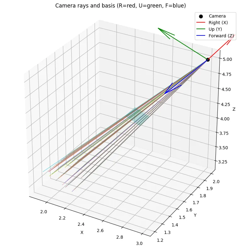
So we first transform our points from Image → Camera space, then multiply the camera directions with the aptly named camera-to-world matrix to get these directions in world coordinates. If you're interested in the exact details, you can check out this explanation. However, in any project where you deal with 3D objects, it's always best to visualize your data to verify everything is working correctly. There are many subtle pitfalls in 3D transformations.

visualization

Now that we’ve our ray positions and directions, we can move on and generate samples across these rays. This is a scalar implementation, as an exercise you can try to vectorize this code.

def stratified_sampling(near, far, N_samples, device='cpu'):
    """
    Inputs:
        near (float): Near bound of the ray (start distance)
        far (float): Far bound of the ray (end distance)  
        N_samples (int): Number of sample points along each ray
        device (str): Device to create tensors on
    """
    # Create evenly spaced bins between near and far
    t_vals = torch.linspace(0.0, 1.0, N_samples, device=device)
   
    # Convert from [0,1] to [near, far] range
    z_vals = near * (1.0 - t_vals) + far * t_vals  # Shape: (N_samples,)
   
    bin_width = (far - near) / N_samples
   
    # Generate random offsets within each bin
    jitter = torch.rand_like(z_vals) * bin_width
   
    # Apply the jitter to get our final sample positions
    z_vals = z_vals + jitter
   
    return z_vals

Let’s use this function to create our data batches. We start with rays_origin, rays_direction and z_vals which have the shapes [10,10, 1, 3] , [10, 10, 1, 3] and [10, 10, 64, 1] where z_vals are generated by using the sampling function above for each pixel. We then create our sample points:

sample_points = rays_o_expanded + z_vals_expanded * rays_d_expanded # [10, 10, 64, 3]

Then the viewing direction for all rays:

view_dirs = rays_d.unsqueeze(-2).expand(-1, -1, N_samples, -1) # [10, 10, 64, 3] 
view_dirs = view_dirs / torch.norm(view_dirs, dim=-1, keepdim=True)

And reshape, encode and run the points through the model:

sample_points_flat = sample_points.reshape(-1, 3) # [6400, 3] 
view_dirs_flat = view_dirs.reshape(-1, 3) # [6400, 3] 
z_vals_flat = z_vals.reshape(-1, N_samples) # [100, 64]

pos_encoded = positional_encoding(sample_points_flat, L=10) # [6400, 60] 
dir_encoded = positional_encoding(view_dirs_flat, L=4) # [6400, 24]

# colors[6400, 3], densities: [6400, 1]
colors, densities = nerf_model(pos_encoded, dir_encoded)

Now reshaping the colors and densities to [10,10,64,3] and [10, 10, 64, 1] as well as the z_vals and ray_direction of shape [10, 10, 64] and [10, 10, 3] respectively we can use the volume rendering formula to write our function.

def volume_render_vectorized(rgb, density, z_vals, rays_d):
    """
    Inputs:
        rgb: [H, W, N_samples, 3] - colors at sample points
        density: [H, W, N_samples, 1] - densities at sample points  
        z_vals: [H, W, N_samples] - distances along rays
        rays_d: [H, W, 3] - ray directions (normalized)
    """
    # Calculate distances between adjacent samples
    dists = z_vals[..., 1:] - z_vals[..., :-1]  # [H, W, N_samples-1]
   
    # Add large distance for last sample (infinity)
    inf_dist = torch.full_like(dists[..., :1], 1e10)  # [H, W, 1]
    dists = torch.cat([dists, inf_dist], dim=-1)  # [H, W, N_samples]
   
    # Calculate alpha vals
    alpha = 1.0 - torch.exp(-density.squeeze(-1) * dists)  # [H, W, N_samples]
   
    # Calculate transmittance following the formula
    optical_depth = density.squeeze(-1) * dists  # [H, W, N_samples]
    cumulative_optical_depth = torch.cumsum(optical_depth, dim=-1)  # [H, W, N_samples]
   
    # T_0 is 1 because camera gets all the light from the first hit point
    transmittance = torch.cat([
        torch.ones_like(cumulative_optical_depth[..., :1]),  # T_0 = 1
        torch.exp(-cumulative_optical_depth[..., :-1])       # T_i = exp(-∑ optical_depth)
    ], dim=-1)
   
    # Weights = (1-exp(-sigma_i * delta_i)) * T_i
    weights = alpha * cumulative_optical_depth  # [H, W, N_samples]
    rgb_final = torch.sum(weights.unsqueeze(-1) * rgb, dim=-2)  # [H, W, 3]
   
    return rgb_final, weights

The output rgb_final and weights would have the shape [10, 10, 3] and [10, 10, 64]. And now since we have predicted RGB colors for each pixel we can simply do a L2 loss between the predicted and the ground truth pixel colors.

Some use cases of NeRFs

There are some great tools online that provide simplified APIs to write efficient pipelines and train your own NeRFs like the NeRF Studio. Take a look at it, I had a lot of fun experimenting with it.

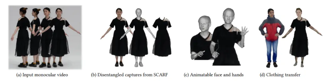
The paper SCARF uses a NeRF to create an avatar where the body and the clothing are disentangled. The body is represented by a traditional mesh, while the clothing is represented by an implicit neural representation using a NeRF.

scarf

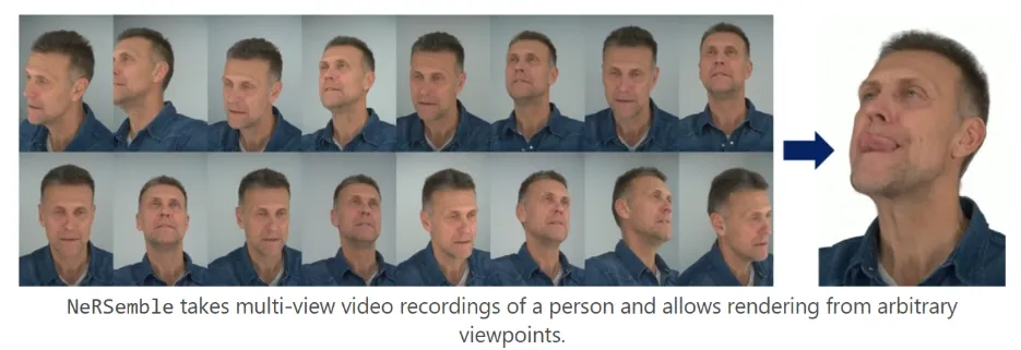
The paper NeRSemble reconstructs high-fidelity radiance fields of human heads while capturing their animations over time and synthesizing renders from novel viewpoints at arbitrary time steps.

nersemble

There are many more examples of NeRFs in action, even though the spotlight got stolen by the Gaussian Splatting approach in recent years.

Textrue

Neural Rendering Adventures #1: NeRFs

Neural Radiance Fields

Optimizing the NeRF

Coding Parts of the Pipeline

Some use cases of NeRFs

References